淘宝用户行为分析「总结」 Alibaba Taobao User Behaviors Analysis All-in-One
Author: Zizhun Guo
作者:
写于:
- 1. Dataset: User Behavior Data from Taobao for Recommendation
- 2. Dateset preprocessing
- 3. Acquisition
- 4. Activation
- 5. Retention
- 6. Revenue
- 7. Recency, frequency, monetary value (RFM) Model
- 8. User Journey
Taobao (Chinese: 淘宝网) is a Chinese online shopping platform. It is headquartered in Hangzhou and owned by Alibaba. It is ranked as the eighth most-visited website. Taobao.com was registered on April 21, 2003 by Alibaba Cloud Computing (Beijing) Co., Ltd.
Taobao Marketplace facilitates consumer-to-consumer (C2C) retail by providing a platform for small businesses and individual entrepreneurs to open online stores that mainly cater to consumers in Chinese-speaking regions (Mainland China, Hong Kong, Macau and Taiwan) and abroad,[4] which is made payable by online accounts. Its stores usually offer an express delivery service.
1. Dataset: User Behavior Data from Taobao for Recommendation
Introduction
The dataset is collected from Tianchi - Data Science Workshop from Aliyun(阿里云)- literally means Alibaba Cloud, the cloud computing service ranked third-largest infrastucture as a service provider, right behind Amazon Web Services, Microsoft Azure.
User Behavior is a dataset of user behaviors from Taobao, for recommendation problem with implicit feedback. The dataset is offered by Alibaba.
| File | Description | Feature |
|---|---|---|
| UserBehavior.csv | All user behavior data | User ID, item ID, category ID, behavior type, timestamp |
UserBehavior.csv
We random select about 1 million users who have behaviors including click, purchase, adding item to shopping cart and item favoring during November 25 to December 03, 2017. The dataset is organized in a very similar form to MovieLens-20M, i.e., each line represents a specific user-item interaction, which consists of user ID, item ID, item’s category ID, behavior type and timestamp, separated by commas. The detailed descriptions of each field are as follows:
| Field | Explanation |
|---|---|
| User ID | An integer, the serialized ID that represents a user |
| Item ID | An integer, the serialized ID that represents an item |
| Category ID | An integer, the serialized ID that represents the category which the corresponding item belongs to |
| Behavior type | A string, enum-type from (‘pv’, ‘buy’, ‘cart’, ‘fav’) |
| Timestamp | An integer, the timestamp of the behavior |
Note that the dataset contains 4 different types of behaviors, they are
| Behavior | Explanation |
|---|---|
| pv | Page view of an item’s detail page, equivalent to an item click |
| fav | Purchase an item |
| cart | Add an item to shopping cart |
| buy | Favor an item |
Dimensions of the dataset are
| Dimension | Number |
|---|---|
| # of users | 987,994 |
| # of items | 4,162,024 |
| # of categories | 9,439 |
| # of interactions | 100,150,807 |
2. Dateset preprocessing
Load the CSV dataset as Spark DateFrame using Pyspark
import findspark
findspark.init('/home/zizhun/spark-3.1.1-bin-hadoop2.7')
from pyspark.sql import SparkSession

# Load csv file into spark dataframe
df = spark.read.csv('UserBehavior.csv')

# Change field names
df = df.withColumnRenamed("_c0","user_id") \
        .withColumnRenamed("_c1","item_id") \
        .withColumnRenamed("_c2","category_id") \
        .withColumnRenamed("_c3","behavior") \
        .withColumnRenamed("_c4","timestamps")
Check out the schema and partial view
root
 |-- user_id: string (nullable = true)
 |-- item_id: string (nullable = true)
 |-- category_id: string (nullable = true)
 |-- behavior: string (nullable = true)
 |-- timestamps: string (nullable = true)

+-------+-------+-----------+--------+----------+
|user_id|item_id|category_id|behavior|timestamps|
+-------+-------+-----------+--------+----------+
|      1|2268318|    2520377|      pv|1511544070|
|      1|2333346|    2520771|      pv|1511561733|
|      1|2576651|     149192|      pv|1511572885|
|      1|3830808|    4181361|      pv|1511593493|
|      1|4365585|    2520377|      pv|1511596146|
|      1|4606018|    2735466|      pv|1511616481|
|      1| 230380|     411153|      pv|1511644942|
|      1|3827899|    2920476|      pv|1511713473|
|      1|3745169|    2891509|      pv|1511725471|
|      1|1531036|    2920476|      pv|1511733732|
+-------+-------+-----------+--------+----------+
only showing top 10 rows
Transform timestamps from Unixtime to date The original timestamp is in format of Unixtime, therefore transforming it into 6 new readable field as datetime, date, month, day, hour and dayofweek.
from pyspark.sql.functions import (dayofmonth, hour,
                                  dayofyear,month, dayofmonth,
                                  year,weekofyear,
                                  format_number, date_format, to_date, dayofweek)

df1.select(dayofmonth(df1.datetime)).show()

df1 = df1.withColumn('date', to_date(df1.datetime)) \
            .withColumn('month', month(df1.datetime)) \
            .withColumn('day', dayofmonth(df1.datetime)) \
            .withColumn('hour', hour(df1.datetime)) \
            .withColumn('dayofweek', dayofweek(df1.datetime))
Results:
+-------+-------+-----------+--------+----------+-------------------+----------+-----+---+----+---------+
|user_id|item_id|category_id|behavior|timestamps|           datetime|      date|month|day|hour|dayofweek|
+-------+-------+-----------+--------+----------+-------------------+----------+-----+---+----+---------+
|      1|2268318|    2520377|      pv|1511544070|2017-11-24 12:21:10|2017-11-24|   11| 24|  12|        6|
|      1|2333346|    2520771|      pv|1511561733|2017-11-24 17:15:33|2017-11-24|   11| 24|  17|        6|
|      1|2576651|     149192|      pv|1511572885|2017-11-24 20:21:25|2017-11-24|   11| 24|  20|        6|
|      1|3830808|    4181361|      pv|1511593493|2017-11-25 02:04:53|2017-11-25|   11| 25|   2|        7|
|      1|4365585|    2520377|      pv|1511596146|2017-11-25 02:49:06|2017-11-25|   11| 25|   2|        7|
|      1|4606018|    2735466|      pv|1511616481|2017-11-25 08:28:01|2017-11-25|   11| 25|   8|        7|
|      1| 230380|     411153|      pv|1511644942|2017-11-25 16:22:22|2017-11-25|   11| 25|  16|        7|
|      1|3827899|    2920476|      pv|1511713473|2017-11-26 11:24:33|2017-11-26|   11| 26|  11|        1|
|      1|3745169|    2891509|      pv|1511725471|2017-11-26 14:44:31|2017-11-26|   11| 26|  14|        1|
|      1|1531036|    2920476|      pv|1511733732|2017-11-26 17:02:12|2017-11-26|   11| 26|  17|        1|
+-------+-------+-----------+--------+----------+-------------------+----------+-----+---+----+---------+
only showing top 10 rows
Discover dataset on the range of date
SELECT Date, n_interactions
FROM
    (SELECT date as Date, COUNT(user_id) as n_interactions
    FROM taobao
    GROUP BY date
    ORDER BY date)
WHERE n_interactions > 10000
         Date  n_interactions
0  2017-11-24         3453235
1  2017-11-25        10598765
2  2017-11-26        10496631
3  2017-11-27         9985084
4  2017-11-28         9987905
5  2017-11-29        10350799
6  2017-11-30        10542266
7  2017-12-01        11712571
8  2017-12-02        14057989
9  2017-12-03         8946657
The distribution shows most of the interactions are conducted between 2017-11-24 to 2017-12-03 (10 days).
Create TempView as Taobao from records based on the distribution
df1.createOrReplaceTempView("taobao")
3. Acquisition
The point for Acquisition analysis is to develop knowledge about the ability of the product to convert visitors into customers. It helps evaluate the efficiency of the business process. The product may have diverse marketing sources of visitors and different channels to fulfill the conversion.
In Taobao user behavior dataset, the ‘behavior’ field can be intuitively interpreted owning the values in an ordinal nature, since the business allows provide purchasing behaviors which are able to independently conducted, e.g. users can choose to purchase the item directly or put it into the cart or favorites. Therefore, there are multiple channels that convert the item visit into the final order. Hence, I take multiple funnel analyses to study its acquisitional traits.
Global Page View (PV), Unique User (UV), PV/UV
# Pychart can query records using Dataframe SQL functions

from pyspark.sql.functions import count, countDistinct
df1.select(countDistinct(df1.user_id).alias('uv')).show()
+------+
|    uv|
+------+
|987991|
+------+
The dataset has 987,991 unique users. Hence, UV = 987,991.
# The same, group by on 'behavior' and find the count for the 'pv'

df1.groupby('behavior').count().orderBy('count', ascending = False).show()
+--------+--------+
|behavior|   count|
+--------+--------+
|      pv|89697359|
|    cart| 5530446|
|     fav| 2888258|
|     buy| 2015839|
+--------+--------+
The dataset has 89,697,359 page view behaviors between 2017-11-24 to 2017-12-03. Hence, PV = 89,697,359.
The PV/UV, the average page view per user evaluates the popularity for the items to be seen in a global sense. We could calculate it for each item. However, this metric needs to be used with other global metrics.
The PV/UV is 90. In these 10 days, the average page views for each unique user is 90.
Bounce Rate
Bounce rate is single-page sessions divided by all sessions, or the percentage of all sessions on the site in which users viewed only a single page and triggered only a single request to the Analytics server. - reference
In the Taobao user behavior case, the unique users who visit items once during the 10-day session would be only considered. Therefore, this bounce rate evaluates the attractiveness of the website instead of a specific item.
Create
# Create TempView with the user count for the different behavior.
# PK: user_id
spark.sql("""
SELECT
    user_id,
    SUM(case when behavior='pv' then 1 else 0 end) as PageView,
    SUM(case when behavior='fav' then 1 else 0 end) as Favorite,
    SUM(case when behavior='cart' then 1 else 0 end) as Cart,
    SUM(case when behavior='buy' then 1 else 0 end) as Buy
FROM
    taobao
GROUP BY
    user_id
""").createTempView("behaviorCount")

spark.sql("""
SELECT
    COUNT(user_id)
FROM
    behaviorCount
WHERE PageView = 1 AND Favorite = 0 AND Cart = 0 AND Buy = 0;
""").show()
+-----------------------+
|count(DISTINCT user_id)|
+-----------------------+
|                     53|
+-----------------------+
The number of unique users who have only 1 page view count is 53. The bounce rate, 53/UV is 0.0053%. It is very small, it proves the visitors, no matter new or old, would not stop discovering the website at the first sight.
Conversion Rate (CVR)
The conversion rate is the percentage of visitors to the website that complete a desired goal (a conversion) out of the total number of visitors.-[Source]
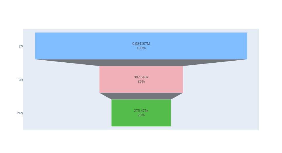
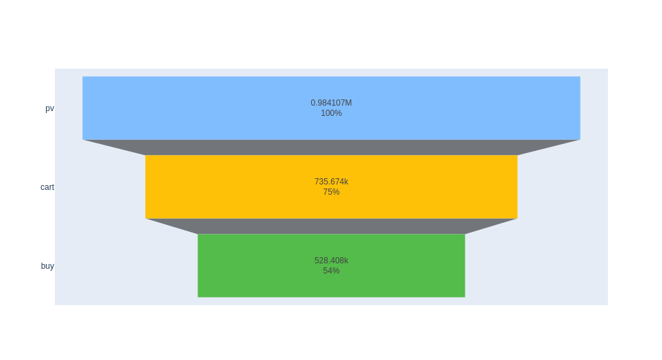
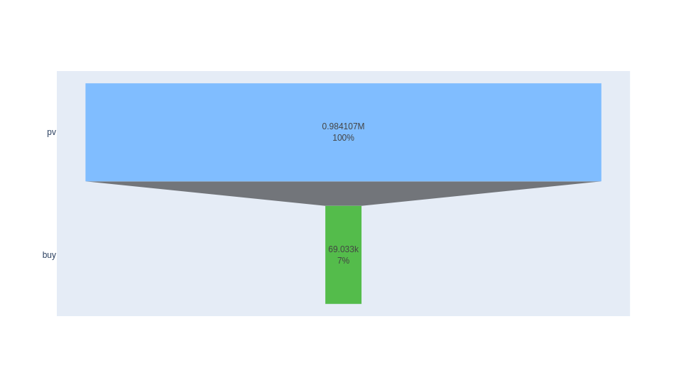
The desired goal is make-purchase. There are three channels to make such conversion (see fig 1 below): 1. page view - favorite - buy; 2. page view - cart - buy; 3. page view - buy. Each channel can conduct a funnel analysis.
pv - fav - buy
CVR for page view user to favorite user = # of users who have pv and fav/ # of users who have pv
n_unique_fav_users = spark.sql("""
SELECT COUNT(DISTINCT user_id)
FROM behaviorCount
WHERE PageView > 0 AND Favorite > 0
""").collect()[0][0] # 387548

n_unique_pv_users = spark.sql("""
SELECT COUNT(DISTINCT user_id)
FROM behaviorCount
WHERE PageView > 0
""").collect()[0][0] # 984107

CVR_pv2fav = n_unique_fav_users/n_unique_pv_users # 387548/984107
The conversion rate for pv to fav is 39.38%.
CVR for page view user to favorite to buy user = # of users who have pv, fav and buy / # of users who have pv
n_unique_fav_buy_users = spark.sql("""
SELECT COUNT(DISTINCT user_id)
FROM behaviorCount
WHERE PageView > 0 AND Favorite > 0 AND Buy > 0
""").collect()[0][0] # 275476

CVR_pv2fav2buy = n_unique_fav_buy_users / n_unique_pv_users # 275476 / 984107
print(CVR_pv2fav2buy)
The conversion rate for pv-fav-buy is 27.99%.
pv - cart - buy
CVR for page view user to cart user = # of users who have pv and cart / # of users who have pv
n_unique_cart_users = spark.sql("""
SELECT COUNT(DISTINCT user_id)
FROM behaviorCount
WHERE PageView > 0 AND Cart > 0
""").collect()[0][0] # 735674

CVR_pv2cart = n_unique_cart_users / n_unique_pv_users # 735674 / 984107
print(CVR_pv2cart)
The conversion rate for pv-cart is 74.56%.
CVR for page view user to cart to buy user = # of users who have pv, cart and buy / # of users who have pv
n_unique_cart_buy_users = spark.sql("""
SELECT COUNT(DISTINCT user_id)
FROM behaviorCount
WHERE PageView > 0 AND Cart > 0 AND Buy > 0
""").collect()[0][0] # 528408

CVR_pv2cart2buy = n_unique_cart_buy_users / n_unique_pv_users # 528408 / 984107
print(CVR_pv2cart2buy)
The conversion rate for pv-cart-buy is 53.69%.
pv - buy
CVR for page view user to buy user = # of users who have pv and buy / # of users who have pv
n_unique_pv_buy_users = spark.sql("""
SELECT COUNT(DISTINCT user_id)
FROM behaviorCount
WHERE PageView > 0 AND Favorite = 0 AND Cart = 0 AND Buy > 0
""").collect()[0][0]

CVR_pv2buy = n_unique_pv_buy_users / n_unique_pv_users
print(CVR_pv2buy)
The conversion rate for pv-buy is 7.01%. (There might have users who have both pv-buy or pv-fav/cart-buy behaviors, such SQL would exclude those users who have both behaviors, therefore the CVR for pv-buy would be higher if based on items)
Funnel plot for 3 channels based on # of users
from plotly import graph_objects as go

fig1 = go.Figure(go.Funnel(
    y = ['pv', 'fav', 'buy'],
    x = [n_unique_pv_users, n_unique_fav_users, n_unique_fav_buy_users],
    textposition = "inside",
    textinfo = "value+percent initial",
    marker = {"color": ["#80bdff", "#f1b0b7", "#54bc4b"]})
    )
fig1.show()
4. Activation
The Activation evaluates the Ecommerce’s ability to provide users with the “Aha moment”. It overlaps the concept with the acquisition a little, but the difference is that the activation focuses on the micro-conversion part whereas users are having enjoyable and solid experiences in the individual part of the product process.
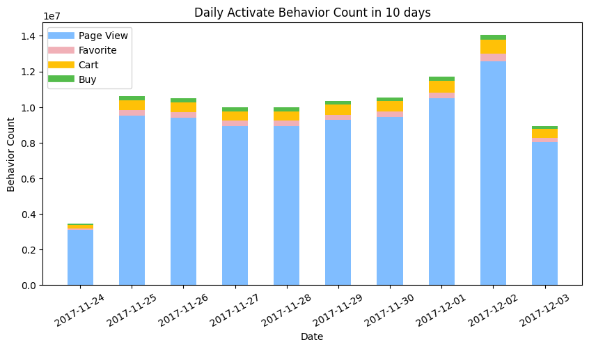
Daily Active behaviors distribution
Details aside, first look at the distribution for the number of daily behaviors between 2017-11-24 to 2017-12-03.
df_date_behavior_count = spark.sql("""
SELECT
    date,
    SUM(CASE WHEN behavior = 'pv' THEN 1 ELSE 0 END) AS pv,
    SUM(CASE WHEN behavior = 'fav' THEN 1 ELSE 0 END) AS fav,
    SUM(CASE WHEN behavior = 'cart' THEN 1 ELSE 0 END) AS cart,
    SUM(CASE WHEN behavior = 'buy' THEN 1 ELSE 0 END) AS buy
FROM
    taobao
GROUP BY
    date
ORDER BY date
""").toPandas()

print(df_date_behavior_count)
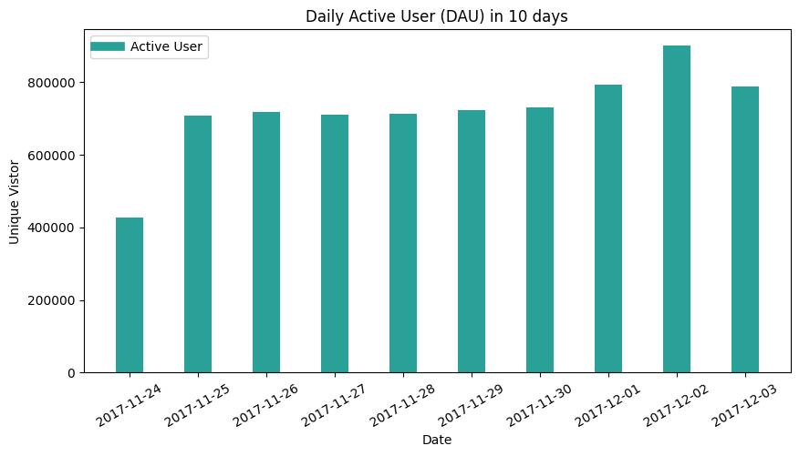
- The number of page view behaviors overwhelmed the other three behaviors favorite, cart, and buy.
- The day of the week for 2017-11-24 is Friday in Beijing Time (GMT+8), whereas it has 13 hours jet leg from US Eastern Time (GMT-5) in winter. It is weird to find that the behavior count on 11-24 is much smaller than 12-01. An assumption to this phenomenon is when binning the behaviors, the part of behaviors conducted in 2017-11-25 morning in china was grouped into the 2017-11-24 in American Time zone, hence the current bars should be moved 1 day after and the value for each date should be partially tunned one by one.
- The current histogram cannot quantitively confirm the relation of behavior count between days, but the trend can be guessed out. After modification, the number of behaviors on Saturday and Sunday is higher than on weekdays.
Daily Active Users(DAU) distribution
df_DAU = spark.sql("""
SELECT
    date,
    COUNT(DISTINCT user_id) AS DAU
FROM
    taobao
GROUP BY
    date
ORDER BY
    date
""").toPandas()

print(df_DAU)
- As to count the unique users in these 10 days, the criteria is any user who conducted one of four behavior count as one active user. Therefore, the relation between DAU to daily active behaviors is similar to the relationship between global unique user numbers and global behavior numbers.
- The trend is similar to DAU histogram, as the time leg and Unix Time function rule still work poorly on a dataset collected from another time zone. The part of unique users is supposed to be grouped on the day after.
Hourly Active Behaviors distribution
df_hour_behavior_count = spark.sql("""
SELECT
    hour,
    SUM(CASE WHEN behavior = 'pv' THEN 0.1 ELSE 0 END) AS pv,
    SUM(CASE WHEN behavior = 'fav' THEN 0.1 ELSE 0 END) AS fav,
    SUM(CASE WHEN behavior = 'cart' THEN 0.1 ELSE 0 END) AS cart,
    SUM(CASE WHEN behavior = 'buy' THEN 0.1 ELSE 0 END) AS buy
FROM
    taobao
WHERE date < '2017-12-04' AND date > '2017-11-23'
GROUP BY
    hour
ORDER BY
    hour
""").toPandas()
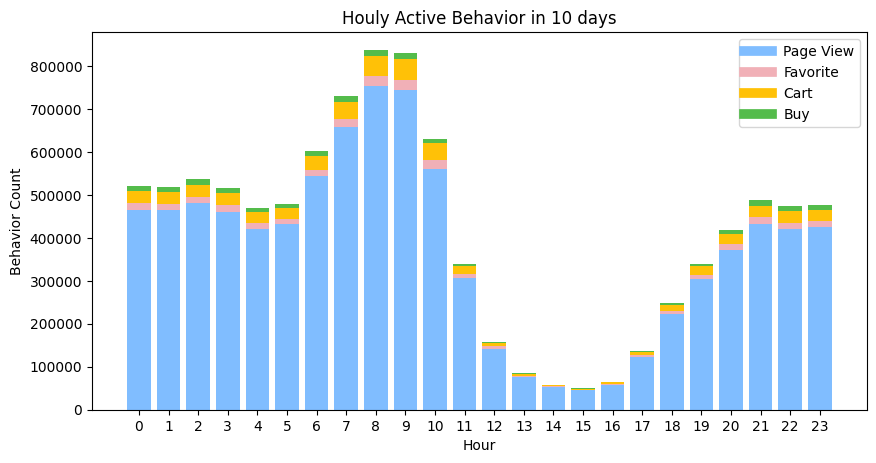
- The distribution is binned by the hour attribute from the table, as it is calculated by averaging the behavior count across 10 days, it compensates for the difference between days.
- The hour illustrates the parsed UNIX time in the American time zone, so there is 13 hours time lag for the real hour within a day scenario. e.g. The 7:00 in US eastern time indicates the 20:00 in the Beijing time zone.
- Based on 2, the peak found between 6:00 to 10:00, when the most popular product using time, is 7 pm to 11 pm in China. It makes sense since this is the time when people get off work and spend time online shopping.
- The behavior count in peak say 9 pm (8:00) is 800k round own, whereas at 4 am (15:00) in the morning, the count is almost only 50k. There are 16 times between the peak and bottom. In day times, the average behavior count is around 500k.
- The rate of decline from peak to bottom is great. It is a common bedtime and people go to sleep quickly. However, once wake up, the usage recovers a bit slower hence users have different things to do.
Hourly Active Users distribution
df_AverageHAU = spark.sql("""
SELECT
    hour,
    ROUND(COUNT(DISTINCT user_id)/10, 0) AS Average_HAU
FROM
    taobao
WHERE date < '2017-12-04' AND date > '2017-11-23'
GROUP BY
    hour
ORDER BY hour
""").toPandas()
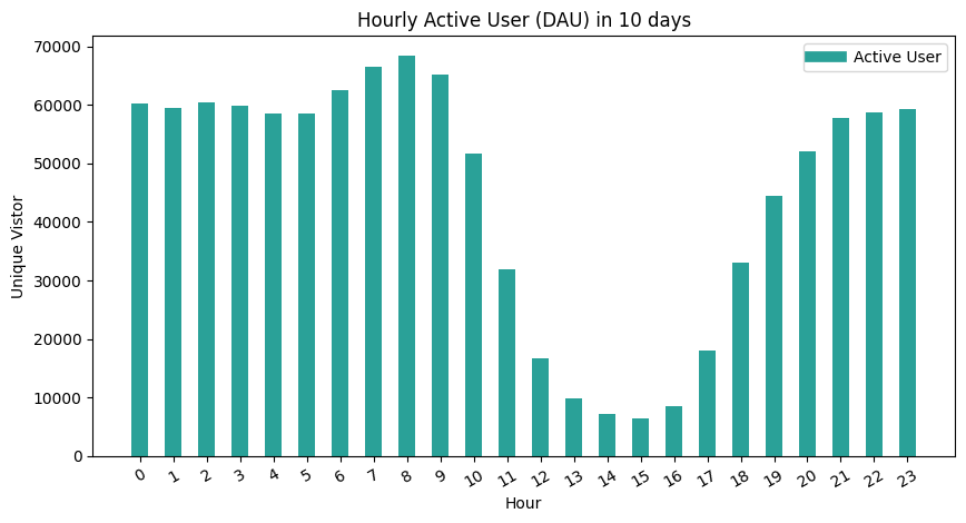
- The trend is similar to hourly behavior count. However, the peak is not as significant as the last one. This indicates that the contribution for unique users on behaviors is not balanced. Given that the trend is similar (same shape), therefore the aspect for causing the balancing issue is that users who are active in the daytime conduct more behaviors at night. It intuitively may make sense that people work in the daytime and get hard to shop online, but at night, they have more time and convenience to use the APP.
- The max value of peak is around 70k whereas the value for the bottom is around 5k, the 12 times difference is greater than 13 times for the behavior count. This indicates the at least for two periods of time (7 pm to 10 pm and 12 am to 5 am), users’ behaviors are normally equalized which helps understand combined with the first point that the users in the daytime are less efficient (number of behaviors per user) than at night.
5. Retention
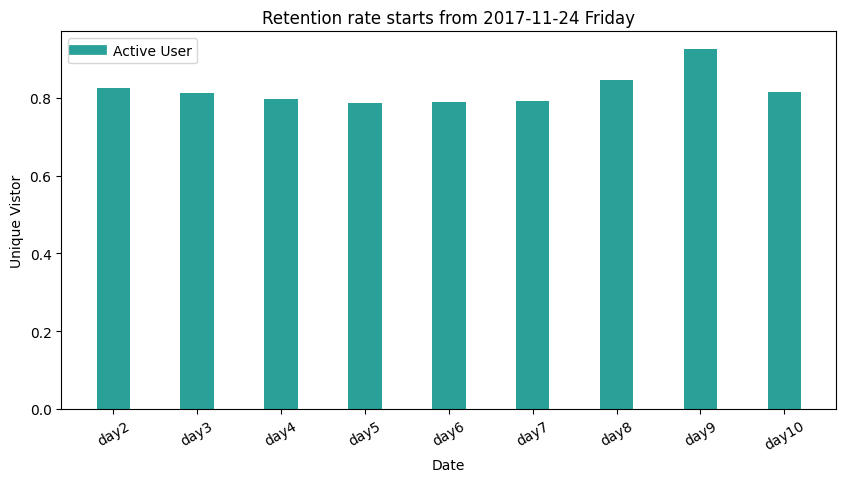
Retention Rate
Retention rate formula: The # of active users continuing to subscribe divided by the total active users at the start of a period = retention rate. [-[Source])(https://www.profitwell.com/customer-retention/calculate-retention-rate)]
The concept to have retention rate metric in a marketing atmosphere is to monitor firm performance in attracting and retaining customers. [-Wikipedia] It is similar to churn rate.
This part of Taobao user behavior analysis technically only provides practice on calculating retention rate metric, since there are no attributes identifying the new users, therefore the users who are count as the first-day user may of the old user, which should not be considered.
df_retention = spark.sql("""
    SELECT
        SUM(CASE WHEN day1 > 0 then 1 else 0 end) AS day1,
        SUM(CASE WHEN day1 > 0 AND day2 > 0 then 1 else 0 end) AS day2retention,
        SUM(CASE WHEN day1 > 0 AND day3 > 0 then 1 else 0 end) AS day3retention,
        SUM(CASE WHEN day1 > 0 AND day4 > 0 then 1 else 0 end) AS day4retention,
        SUM(CASE WHEN day1 > 0 AND day5 > 0 then 1 else 0 end) AS day5retention,
        SUM(CASE WHEN day1 > 0 AND day6 > 0 then 1 else 0 end) AS day6retention,
        SUM(CASE WHEN day1 > 0 AND day7 > 0 then 1 else 0 end) AS day7retention,
        SUM(CASE WHEN day1 > 0 AND day8 > 0 then 1 else 0 end) AS day8retention,
        SUM(CASE WHEN day1 > 0 AND day9 > 0 then 1 else 0 end) AS day9retention,
        SUM(CASE WHEN day1 > 0 AND day10 > 0 then 1 else 0 end) AS day10retention
    FROM
        (SELECT
            user_id,
            SUM(CASE WHEN date = '2017-11-24' then 1 else 0 end) as day1,
            SUM(CASE WHEN date = '2017-11-25' then 1 else 0 end) as day2,
            SUM(CASE WHEN date = '2017-11-26' then 1 else 0 end) as day3,
            SUM(CASE WHEN date = '2017-11-27' then 1 else 0 end) as day4,
            SUM(CASE WHEN date = '2017-11-28' then 1 else 0 end) as day5,
            SUM(CASE WHEN date = '2017-11-29' then 1 else 0 end) as day6,
            SUM(CASE WHEN date = '2017-11-30' then 1 else 0 end) as day7,
            SUM(CASE WHEN date = '2017-12-01' then 1 else 0 end) as day8,
            SUM(CASE WHEN date = '2017-12-02' then 1 else 0 end) as day9,
            SUM(CASE WHEN date = '2017-12-03' then 1 else 0 end) as day10
        FROM taobao
        GROUP BY
            user_id)
    """).toPandas()
Repurchase Rate
Repurchase rate is the percentage rate of a cohort having placed another order within a certain period of time, typically calculated within 30/60/90/180/360 days from the first order. [-Source]
Due to the limit of time periods, we calculate the 10-day repurchase rate. The way to calculate it is to find the number of unique users who have purchased twice within 10 days.
n_repurchase = spark.sql("""
SELECT COUNT(DISTINCT user_id)
FROM
    (SELECT user_id, COUNT(behavior) AS buy_times
    FROM taobao
    WHERE behavior = 'buy'
    GROUP BY
        user_id)
WHERE buy_times > 1
""").collect()[0][0]

n_purchase = spark.sql("""
SELECT COUNT(DISTINCT user_id)
FROM
    (SELECT user_id, COUNT(behavior) AS buy_times
    FROM taobao
    behavior = 'buy'
    GROUP BY
        user_id)
""").collect()[0][0]

print(n_repurchase/n_purchase)
The repurchase rate is 66%.
There is another way to calculate which is by finding the count of unique users number who has conducted another transaction within the 10 days except for the first day.
6. Revenue
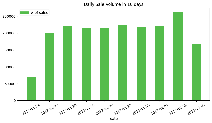
A transaction is made by users conducting a buy behavior, defined by this analysis. No matter the order is completely fulfilled or not. In fact, a metric called Gross Merchandise Volume (GMV) is used to evaluate the total gross income within a period of time. Unfortunately, the table does not contain the price feature for items, therefore we only calculate the total sale volume in dates and rank them group by the item category and items themselves.
Daily Sale Volume in 10 days
df_daily_sales_volume = spark.sql("""
SELECT
    date,
    SUM(CASE WHEN behavior = 'pv' then 1 else 0 end) as pv,
    SUM(CASE WHEN behavior = 'fav' then 1 else 0 end) as fav,
    SUM(CASE WHEN behavior = 'cart' then 1 else 0 end) as cart,
    SUM(CASE WHEN behavior = 'buy' then 1 else 0 end) as buy
FROM taobao
GROUP BY
    date
""").toPandas()
As PART II mentioned, due to the parsing issue, the UNIX time collected from GMT+8 time zone is interpreted to GMT-5 time zone, so part of sales conducted on 11-25 are binned to 11-24. One day shift to right, the sale volume based on a date shows a consistent invariance even encountering the weekends.
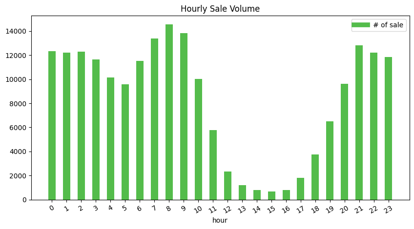
Hourly Sale Volume in 10 days
df_hourly_sales_volume = spark.sql("""
SELECT
    hour,
    SUM(CASE WHEN behavior = 'pv' then 0.1 else 0 end) as pv,
    SUM(CASE WHEN behavior = 'fav' then 0.1 else 0 end) as fav,
    SUM(CASE WHEN behavior = 'cart' then 0.1 else 0 end) as cart,
    SUM(CASE WHEN behavior = 'buy' then 0.1 else 0 end) as buy
FROM taobao
GROUP BY
    hour
ORDER BY
    hour
""").toPandas()
The UNIX time functions from Pyspark make the hour become the US time based on the local machine, so the hour shows in the figure should convert into the Beijing time as the sale are conducted in China region. e.g. 6 pm to 19:00
- Comparing with hourly behaviors distribution, the difference is in the period of time between 3 am (16:00) to 6 pm (19:00), the sale volume has a little decrease among all hours of the day.
- The peak has around 14000 sale volumes whereas the bottom has around 1000 sale volumes. The difference is around 14 times which is the same as the behavior distribution.
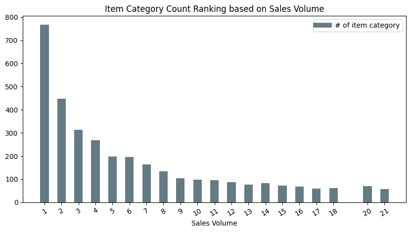
Sales Volume Ranking on item category
df_sales_volume_ranking_category = spark.sql("""
SELECT
    a.buy_times AS sales_volume,
    COUNT(a.category_id) AS category_num
FROM
    (SELECT
        category_id,
        COUNT(user_id) AS buy_times
    FROM
        taobao
    WHERE
        behavior='buy'
    GROUP BY
        category_id ) AS a
GROUP BY
    a.buy_times
ORDER BY
    category_num DESC;
""").toPandas()
sales_volume 	1 	2 	3 	4 	5 	6 	7 	8 	9 	10 	... 	1158 	3096 	18016 	1147 	458 	1326 	2015 	6354 	2782 	2203
category_num 	767 	448 	313 	268 	198 	195 	163 	133 	105 	97 	... 	1 	1 	1 	1 	1 	1 	1 	1 	1 	1
Based on the sale volume, we ranked the item categories’ count. The figure above shows there are almost 800 categories of items are sold only once among all users. The second place’s category of an item which sold twice counts around 450. The overall trend follows a logarithmic pattern in a descending prone.
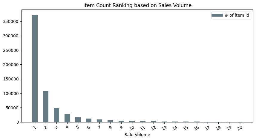
Sales Volume Ranking on item id
df_sales_volume_ranking_item = spark.sql("""
SELECT
    a.buy_times AS sales_volume,
    COUNT(a.item_id) AS item_num
FROM
    (SELECT
        item_id,
        COUNT(user_id) AS buy_times
    FROM
        taobao
    WHERE
        behavior='buy'
    GROUP BY
        item_id ) AS a
GROUP BY
    a.buy_times
ORDER BY
    item_num DESC;
""").toPandas()
The second study on item id ranking based on the sale volume indicates a similar trend as to how it was performed with the item category rank. They both follow a logarithmic declining trend, but for the current item ranking trend, it is deeper. Over 350,000 items are sold once which takes a larger portion, whereas the items sold twice are only take 1/4 in the value.
Item id ranking vs Item category ranking (on Sale Volume)
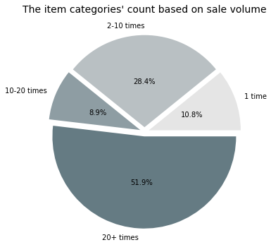
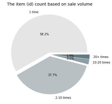
It is interesting to conduct the pie charts for both rankings and compare how much the portions take for different granularity of data tag. Much easy to understand, the category tag has fewer unique values than item id since one category can include multiple items, hence the portion for ranking would be different.
As seen from the figure on the left-hand side, half of the item categories have their belonging items sold 20+ times, as for those less popular item categories, one sold only once still takes 10 percent, these are the super unpopular item category. From the figure on the right-hand side, within the super unpopular item category, the items’ number overwhelmingly populates 58.2 percent among all items. Combined with the items which sold 2-10 times, it is interesting to see that most of the items (96 percent) of items are not popular at all, whereas only 2 percent of items are able to sell at least 20 times, in other words, getting into the transaction order.
For further mining processing, a possible direction is to cluster the item category based on the distribution of its item sale volume. One guess is there might have an item category that has 1 or 2 items specifically popular with almost no visit for the rest, or some item categories may exist that all items belonging to them are regular.
7. Recency, frequency, monetary value (RFM) Model
Recency, frequency, monetary value is a marketing analysis tool used to identify a company’s or an organization’s best customers by using certain measures. The RFM model is based on three quantitative factors:
- Recency: How recently a customer has made a purchase
- Frequency: How often a customer makes a purchase
- Monetary Value: How much money a customer spends on purchases
RFM analysis numerically ranks a customer in each of these three categories, generally on a scale of 1 to 5 (the higher the number, the better the result). The “best” customer would receive a top score in every category.
We take the above approach to category the users based on the rule with the last time buy behavior and frequency of buy behavior. Here are the rules:
R:score the user's recency based on the time difference from the buy behavior date to 17-12-03
difference > 7 score = 1
difference BETWEEN 5-7 score = 2
difference BETWEEN 3-4 score = 3
difference BETWEEN 0-2 score = 4

F:score the user's frequency based on the date of the buy behavior count
purchase once score = 1
purchase twice score = 2
purchase 3-10 times score = 3
purchase times > 10 score = 4
Since the table does not contain monetary info, hence ignore the monetary value.
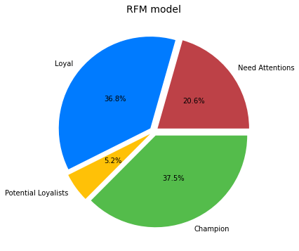
Once having the scores of users’ Recency and Frequency, applying another rule to classify users into different group.
Champion:
FrequencyScore BETWEEN 3-4 AND RecencyScore BETWEEN 3-4

Loyal:
FrequencyScore BETWEEN 3-4 AND RecencyScore BETWEEN 1-2

Potential Loyalists:
FrequencyScore BETWEEN 1-2 AND RecencyScore BETWEEN 3-4

Need Attentions
FrequencyScore BETWEEN 1-2 AND RecencyScore BETWEEN 1-2
spark.sql("""
SELECT
    user_id,
    (CASE WHEN Rdiff >7 THEN 1
    WHEN Rdiff BETWEEN 5 AND 7 THEN 2
    WHEN Rdiff BETWEEN 3 AND 4 THEN 3
    WHEN Rdiff BETWEEN 0 AND 2 THEN 4
    ELSE NULL END ) AS RecencyScore
FROM
    (SELECT
        user_id,
        DATEDIFF('2017-12-03',max(date)) AS Rdiff
    FROM
        taobao
    WHERE
        behavior='buy'
    GROUP BY
        user_id)

""").createOrReplaceTempView("R1")

spark.sql("""
SELECT
    user_id,
    (case WHEN SaleVolume BETWEEN 1 AND 1 THEN 1
    WHEN SaleVolume BETWEEN 2 AND 2 THEN 2
    WHEN SaleVolume BETWEEN 3 AND 10 THEN 3
    WHEN SaleVolume >=11 THEN 4
    ELSE NULL END ) as FrequencyScore
FROM(
    SELECT
        user_id,
        COUNT(behavior) AS SaleVolume
    FROM
        taobao
    WHERE
        behavior='buy'
    GROUP BY
        user_id)
""").createOrReplaceTempView("F1")

df_RFM = spark.sql("""
SELECT
    user_id,
    RecencyScore,
    FrequencyScore,
    (CASE WHEN (FrequencyScore BETWEEN 1 AND 2)AND(RecencyScore BETWEEN 1 AND 2 )THEN 1
    WHEN (FrequencyScore BETWEEN 1 AND 2)AND(RecencyScore BETWEEN 3 AND 4 )THEN 2
    WHEN (FrequencyScore BETWEEN 3 AND 4)AND(RecencyScore BETWEEN 1 AND 2 )THEN 3
    WHEN (FrequencyScore BETWEEN 3 AND 4)AND(RecencyScore BETWEEN 3 AND 4 )THEN 4
    ELSE NULL END ) AS CustomerLevel
FROM
    (SELECT
        R1.user_id,
        R1.RecencyScore,
        F1.FrequencyScore
    FROM
        R1
    INNER JOIN
        F1
    ON
        R1.user_id=F1.user_id)
""").toPandas()

print(df_RFM)
        user_id  RecencyScore  FrequencyScore  CustomerLevel
0       1000240             4               3              4
1       1000280             4               2              2
2       1000665             4               3              4
3       1000795             4               2              2
4       1000839             4               3              4
...         ...           ...             ...            ...
672399   999498             2               1              1
672400   999507             4               3              4
672401   999510             4               3              4
672402   999616             2               1              1
672403   999656             3               1              2

[672404 rows x 4 columns]
8. User Journey
A user journey is the experiences a person has when interacting with something, typically software. User journeys describe at a high level of detail exactly what steps different users take to complete a specific task within a system, application, or website. User journeys are focused on the user and what they see and what they do, in comparison to the related web design term click path which is just a plain list of the text URLs that are hit when a user follows a particular Journey.
The customer journey is divided into five phases which refer to the AIDA model.
- Awareness Awareness for the product is awakened (inspiration)
- Interest The interest in the product is increased (favoritism)
- Desire The customer is considering buying the product (wish)
- Action The product is bought (implementation)
We have found the concept of user journey can be applied to the taobao Dataset. (see Part II conversion analysis) In taobao dataset, it has four behavior types which are page view, favorite, cart and buy. Combining with user_id and item_id, a user journey behavior can be defined as a series of behaviors conducted by a user targeting a specific item. See example below: Table 1: a user journey track
| user_id | item_id | Timestamps | Behavior |
|---|---|---|---|
| 100 | 12345678 | 2017-11-25 13:04:00 | pv |
| 100 | 12345678 | 2017-11-25 13:12:23 | fav |
| 100 | 12345678 | 2017-11-27 10:56:10 | pv |
| 100 | 12345678 | 2017-11-27 20:23:59 | buy |
See table 1 above, a user (id: 100) has viewed a page of the item (id: 12345678) at 2017-11-25 13:04:00. 8 mins later, this user had put this item into the favorite list. Two days later, this user viewed this item again. About 10 hours later, at 8 pm on the same day, this user purchased this item.
Goal
The goal of the task is to use millions of user-journey behaviors to identify customer categories/clusters that can be useful for targeted consumer insights at scale. The tool to implement is Apache Spark: Spark SQL and MLlib. The clustering model is KMeans.
Preprocessing
From part I, most of the behaviors are in dates between 2017-11-24 to 2017-12-03, therefore we select 5,000,000 records of behaviors from the subset of the dataset. Another reason to choose only 5M records instead of the 100M from the original size is that while doing statistic analysis later after KMeans, the virtual machine’s memory (8GM) simply cannot hold the query processing when conducted on the aggregated temporary view, hence only taking part of the dataset.
Feature Engineering: Aggregation
Set up some statistical rules to extract some features from the orignal dataset:
| Rule | Explanation |
|---|---|
| duration | The time difference between the minimal timestamps and maximum timestamps within the user journey |
| behavior_count | The total behavior count of a user journey |
| pv | The pv count of a user journey |
| fav | The fav count of a user journey |
| cart | The cart count of a user journey |
| buy | The buy count of a user journey |
| label | Whether the user have purchased the item or not |
df = spark.sql("""
SELECT
    user_id,
    item_id,
    MAX(timestamps)-MIN(timestamps) as duration,
    COUNT(item_id) as behavior_count,
    SUM(CASE WHEN behavior = 'pv' THEN 1 ELSE 0 END) as pv,
    SUM(CASE WHEN behavior = 'fav' THEN 1 ELSE 0 END) as fav,
    SUM(CASE WHEN behavior = 'cart' THEN 1 ELSE 0 END) as cart,
    SUM(CASE WHEN behavior = 'buy' THEN 1 ELSE 0 END) as buy
FROM taobao
GROUP BY user_id, item_id
ORDER BY user_id, item_id ASC
""")

df.createOrReplaceTempView("taobao_clustering")

df = spark.sql("""
SELECT
    *,
    CASE WHEN buy > 0 THEN 1 ELSE 0 END as label
FROM taobao_clustering
""")

from pyspark.ml.feature import VectorAssembler

assembler = VectorAssembler(inputCols = feat_cols, outputCol = 'features')
final_data = assembler.transform(df)

from pyspark.ml.feature import StandardScaler

scaler = StandardScaler(inputCol = 'features', outputCol = 'scaledFeatures')
scaler_model = scaler.fit(final_data)
cluster_final_data = scaler_model.transform(final_data)
Quick view for the Spark dataframe:
+-------+-------+--------+--------------+---+---+----+---+-----+--------------------+--------------------+
|user_id|item_id|duration|behavior_count| pv|fav|cart|buy|label|            features|      scaledFeatures|
+-------+-------+--------+--------------+---+---+----+---+-----+--------------------+--------------------+
|      1|1305059|     0.0|             1|  1|  0|   0|  0|    0| (7,[1,2],[1.0,1.0])|(7,[1,2],[0.99231...|
|      1|1323189|     0.0|             1|  1|  0|   0|  0|    0| (7,[1,2],[1.0,1.0])|(7,[1,2],[0.99231...|
|      1|1338525|     0.0|             1|  1|  0|   0|  0|    0| (7,[1,2],[1.0,1.0])|(7,[1,2],[0.99231...|
|      1|1340922|     0.0|             1|  1|  0|   0|  0|    0| (7,[1,2],[1.0,1.0])|(7,[1,2],[0.99231...|
|      1|1531036|     0.0|             1|  1|  0|   0|  0|    0| (7,[1,2],[1.0,1.0])|(7,[1,2],[0.99231...|
|      1|2028434|     0.0|             1|  1|  0|   0|  0|    0| (7,[1,2],[1.0,1.0])|(7,[1,2],[0.99231...|
|      1|2041056|     0.0|             1|  1|  0|   0|  0|    0| (7,[1,2],[1.0,1.0])|(7,[1,2],[0.99231...|
|      1|2087357| 29426.0|             2|  2|  0|   0|  0|    0|(7,[0,1,2],[29426...|(7,[0,1,2],[0.347...|
|      1|2104483|     0.0|             1|  1|  0|   0|  0|    0| (7,[1,2],[1.0,1.0])|(7,[1,2],[0.99231...|
|      1|2266567|     0.0|             1|  1|  0|   0|  0|    0| (7,[1,2],[1.0,1.0])|(7,[1,2],[0.99231...|
+-------+-------+--------+--------------+---+---+----+---+-----+--------------------+--------------------+
only showing top 10 rows
Clustering KMeans
Apply KMeans to the scaled dataset with different k values.
KMeans hyperparameters:
| hyperparameter | Value |
|---|---|
| tol | 0.0001 |
| maxIter | 20 |
| distanceMeasure | euclidean |
| weightCol | none |
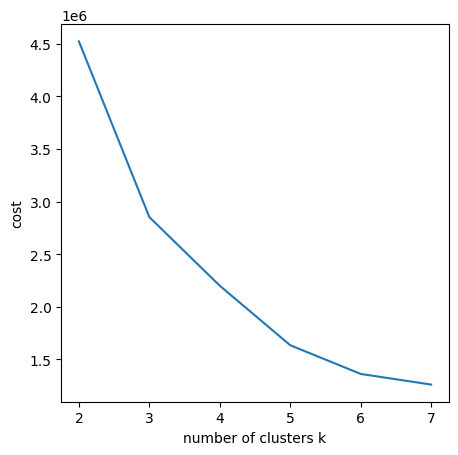
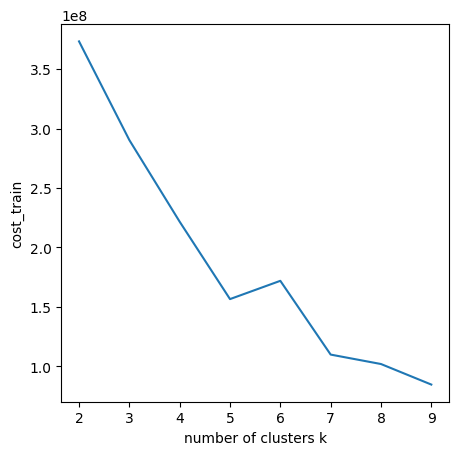
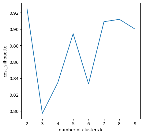
Using Elbow/Knee Method for a quick look-out to select K values.
Looks like k = 3, k = 5 and k = 6 are the good change-points. Select k = 5 as the cluster numbers. Here print out the clustering results. (The ‘prediction’ indicates the cluster number ranged from 0 - 4)
+-------+-------+--------+--------------+---+---+----+---+-----+--------------------+--------------------+----------+
|user_id|item_id|duration|behavior_count| pv|fav|cart|buy|label|            features|      scaledFeatures|prediction|
+-------+-------+--------+--------------+---+---+----+---+-----+--------------------+--------------------+----------+
|      1|1305059|     0.0|             1|  1|  0|   0|  0|    0| (7,[1,2],[1.0,1.0])|(7,[1,2],[0.93053...|         0|
|      1|1323189|     0.0|             1|  1|  0|   0|  0|    0| (7,[1,2],[1.0,1.0])|(7,[1,2],[0.93053...|         0|
|      1|1338525|     0.0|             1|  1|  0|   0|  0|    0| (7,[1,2],[1.0,1.0])|(7,[1,2],[0.93053...|         0|
|      1|1340922|     0.0|             1|  1|  0|   0|  0|    0| (7,[1,2],[1.0,1.0])|(7,[1,2],[0.93053...|         0|
|      1|1531036|     0.0|             1|  1|  0|   0|  0|    0| (7,[1,2],[1.0,1.0])|(7,[1,2],[0.93053...|         0|
|      1|2028434|     0.0|             1|  1|  0|   0|  0|    0| (7,[1,2],[1.0,1.0])|(7,[1,2],[0.93053...|         0|
|      1|2041056|     0.0|             1|  1|  0|   0|  0|    0| (7,[1,2],[1.0,1.0])|(7,[1,2],[0.93053...|         0|
|      1|2087357| 29426.0|             2|  2|  0|   0|  0|    0|(7,[0,1,2],[29426...|(7,[0,1,2],[0.344...|         0|
|      1|2104483|     0.0|             1|  1|  0|   0|  0|    0| (7,[1,2],[1.0,1.0])|(7,[1,2],[0.93053...|         0|
|      1|2266567|     0.0|             1|  1|  0|   0|  0|    0| (7,[1,2],[1.0,1.0])|(7,[1,2],[0.93053...|         0|
|      1|2268318|     0.0|             1|  1|  0|   0|  0|    0| (7,[1,2],[1.0,1.0])|(7,[1,2],[0.93053...|         0|
|      1|2278603|     0.0|             1|  1|  0|   0|  0|    0| (7,[1,2],[1.0,1.0])|(7,[1,2],[0.93053...|         0|
|      1|2286574|     0.0|             1|  1|  0|   0|  0|    0| (7,[1,2],[1.0,1.0])|(7,[1,2],[0.93053...|         0|
|      1| 230380|     0.0|             1|  1|  0|   0|  0|    0| (7,[1,2],[1.0,1.0])|(7,[1,2],[0.93053...|         0|
|      1|2333346|     0.0|             1|  1|  0|   0|  0|    0| (7,[1,2],[1.0,1.0])|(7,[1,2],[0.93053...|         0|
|      1|2576651|     0.0|             1|  1|  0|   0|  0|    0| (7,[1,2],[1.0,1.0])|(7,[1,2],[0.93053...|         0|
|      1| 266784| 25123.0|             2|  2|  0|   0|  0|    0|(7,[0,1,2],[25123...|(7,[0,1,2],[0.294...|         0|
|      1| 271696|     0.0|             1|  1|  0|   0|  0|    0| (7,[1,2],[1.0,1.0])|(7,[1,2],[0.93053...|         0|
|      1|2734026|     0.0|             1|  1|  0|   0|  0|    0| (7,[1,2],[1.0,1.0])|(7,[1,2],[0.93053...|         0|
|      1|2791761|     0.0|             1|  1|  0|   0|  0|    0| (7,[1,2],[1.0,1.0])|(7,[1,2],[0.93053...|         0|
+-------+-------+--------+--------------+---+---+----+---+-----+--------------------+--------------------+----------+
only showing top 20 rows
Statistic Analysis
+-------+-----------------+------------------+------------------+-------------------+-------------------+--------------------+--------------------+------------------+
|summary|         duration|    behavior_count|                pv|                fav|               cart|                 buy|               label|        prediction|
+-------+-----------------+------------------+------------------+-------------------+-------------------+--------------------+--------------------+------------------+
|  count|           756408|            756408|            756408|             756408|             756408|              756408|              756408|            756408|
|   mean|21433.50689707142|1.3220378420111898| 1.184676788188385| 0.0371333989064103|0.07331228649088851|0.026915368425505813|0.025566889826654397|0.4321940011210881|
| stddev|85385.05928533341|1.0746465690895712|0.9953649718484974|0.19056521625685005| 0.2690200842701817| 0.17201339406933566| 0.15783933890990312|1.1010077907100033|
|    min|              0.0|                 1|                 0|                  0|                  0|                   0|                   0|                 0|
|    max|         787426.0|               153|               153|                  7|                  6|                  11|                   1|                 4|
+-------+-----------------+------------------+------------------+-------------------+-------------------+--------------------+--------------------+------------------+
The duration are in seconds unit hence dividing 3600 to convert into hours. The longest duration of the user journey lasts about 9 days. The average duration of the user journey takes around 6 hours.
From label(whether purchased or not) features, it finds 2.5 out of 100 items are eventually purchased. From pv(page view count for each user behavior), we found each item is at least being view once(1.18). Similar findings are documented in the previous part[part II].
Intra-clusters Analysis
Group by the cluster index and calculat the mean values for all features.
df_k5_statistics = spark.sql("""
SELECT prediction AS cluster,
        COUNT(DISTINCT user_id) AS user,
        COUNT(item_id) AS behavior,
        ROUND(AVG(duration)/3600,2) AS avg_duratiion,
        ROUND(AVG(behavior_count),2) as avg_num_behaviors,
        ROUND(AVG(pv),2) as avg_pv,
        ROUND(AVG(fav),2) as avg_fav,
        ROUND(AVG(cart),2) as avg_cart,
        ROUND(AVG(buy),2) as avg_buy,
        ROUND(AVG(label),2) as avg_label
FROM purchase_clustered
GROUP BY prediction
ORDER BY prediction asc
""")
df_k5_statistics.show()
Results:
+-------+----+--------+------------+-----------------+------+-------+--------+-------+---------+
|cluster|user|behavior|avg_duration|avg_num_behaviors|avg_pv|avg_fav|avg_cart|avg_buy|avg_label|
+-------+----+--------+------------+-----------------+------+-------+--------+-------+---------+
|      0|9701|  639437|        0.91|             1.12|  1.12|    0.0|     0.0|    0.0|      0.0|
|      1|6673|   19246|       29.08|             3.08|  1.76|   0.07|     0.2|   1.05|      1.0|
|      2|6688|   28996|       93.98|             3.97|   3.7|   0.05|    0.22|    0.0|      0.0|
|      3|3700|   25239|       10.52|             1.62|  0.58|   1.01|    0.03|    0.0|      0.0|
|      4|6853|   43490|        8.49|             1.61|  0.59|    0.0|    1.02|    0.0|      0.0|
+-------+----+--------+------------+-----------------+------+-------+--------+-------+---------+
Heatmap
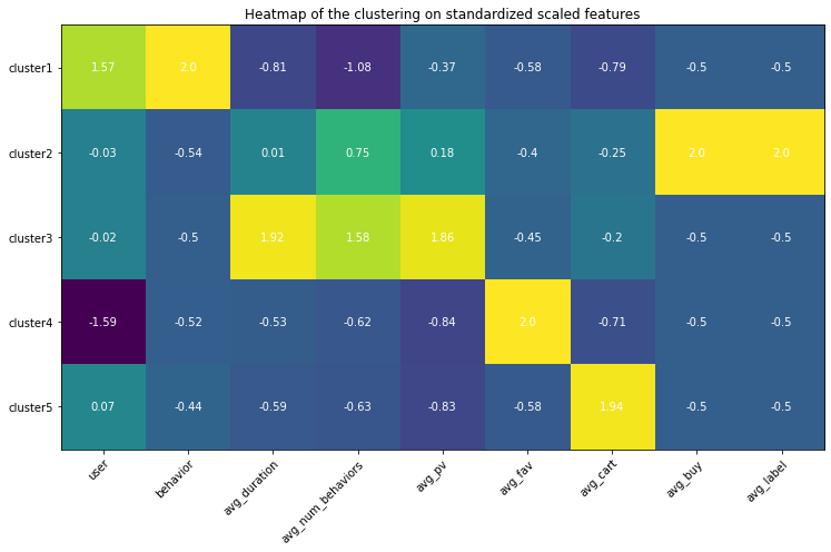
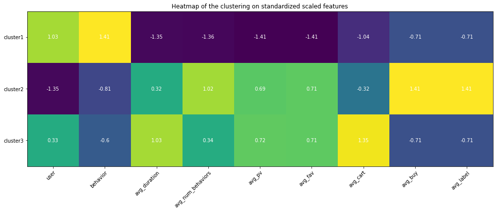
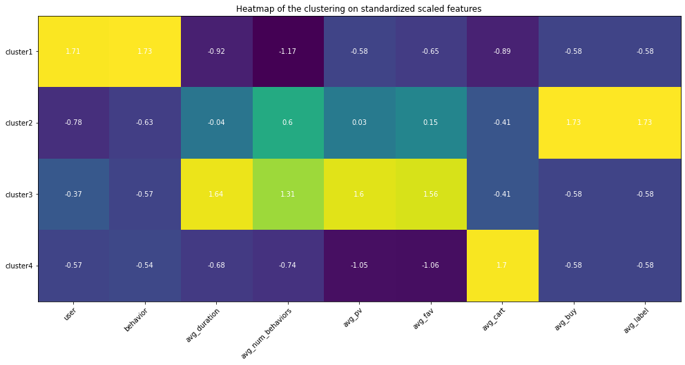
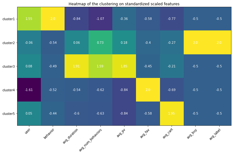
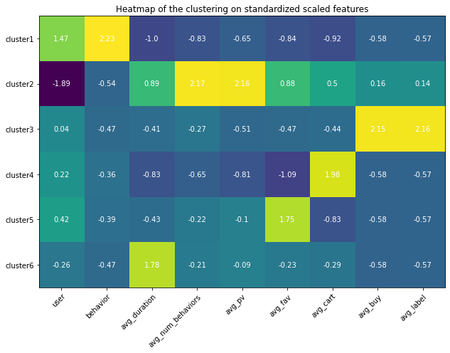
Use heatmap to differentiate among clusters. The highlighted square indicates the feature values are higher than the one from other clusters, which help understand the special traits for that cluster using the domain knowledge.
Use sklearn Standardize features to remove the mean and scale to unit variance.
from sklearn.preprocessing import StandardScaler
scaler = StandardScaler()
scaler.fit(df_k5)
heatmap(np.around(scaler.transform(df_k5), 2))
Analysis based on the heatmap and values
- Cluster 1: this group of behaviors are in high numbers and have the largest number of users involved. However, none of them converts to the final purchase order and they are even unlikely to trigger adding the items to the cart. Among all behavior types, it seems page views are in averages but still, they seem hibernates and less active. The duration between the user journey is the longest.
- Cluster 2: these are the true buyers’ behaviors - averaged user journey duration, above averaged page view count, few carting behaviors, all these behaviors leading to the successfully created purchasing order.
- Cluster 3: these are the active app users’ behavior patterns, almost no purchase at all, but conducting the greatest amount of behaviors in which the most of them are page views. The conversion rate is very low. Maybe the item is too expensive or because of other reasons that users are hesitating. The average user journey duration lasts around 4 days.
- Cluster 4: these behaviors are browsing-focused since there is much less page view amount than the favorite amount, therefore these behaviors are conducted by the browsing pages where the user does not need to click the items’ landing pages but just add the item in the list to the favorites.
- Cluster 5: just like Cluster 4 happened in the users’ browsing process, users directly put items into the cart, and thereafter no further actions were conducted.
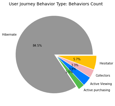
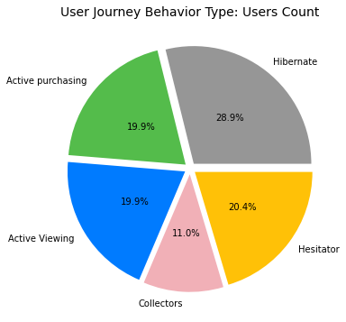
| Cluster | User Journey Behavior Type |
|---|---|
| 1 | Hibernate |
| 2 | Active purchasing |
| 3 | Active Viewing |
| 4 | Collectors |
| 5 | Hesitator |
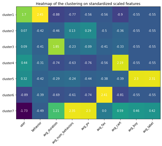
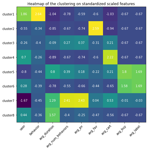
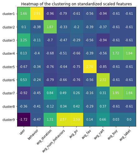
Appendix (Updated 9/19/2021)
Since I had set up my personal cloud workspace, I had successfully fit the entire 100 billion records into the models using PySpark. Here are the updated results:
Copyright @ 2021 Zizhun Guo. All Rights Reserved.


