Alibaba Taobao User Behaviors Analysis IV: AARRR Framework (Revenue) - Sale rank, RFM model annotation
Author: Zizhun Guo
作者:
写于:
1. Recap of the user behavior table
+-------+-------+-----------+--------+----------+-------------------+----------+-----+---+----+---------+
|user_id|item_id|category_id|behavior|timestamps|           datetime|      date|month|day|hour|dayofweek|
+-------+-------+-----------+--------+----------+-------------------+----------+-----+---+----+---------+
|      1|2268318|    2520377|      pv|1511544070|2017-11-24 12:21:10|2017-11-24|   11| 24|  12|        6|
|      1|2333346|    2520771|      pv|1511561733|2017-11-24 17:15:33|2017-11-24|   11| 24|  17|        6|
|      1|2576651|     149192|      pv|1511572885|2017-11-24 20:21:25|2017-11-24|   11| 24|  20|        6|
|      1|3830808|    4181361|      pv|1511593493|2017-11-25 02:04:53|2017-11-25|   11| 25|   2|        7|
|      1|4365585|    2520377|      pv|1511596146|2017-11-25 02:49:06|2017-11-25|   11| 25|   2|        7|
|      1|4606018|    2735466|      pv|1511616481|2017-11-25 08:28:01|2017-11-25|   11| 25|   8|        7|
|      1| 230380|     411153|      pv|1511644942|2017-11-25 16:22:22|2017-11-25|   11| 25|  16|        7|
|      1|3827899|    2920476|      pv|1511713473|2017-11-26 11:24:33|2017-11-26|   11| 26|  11|        1|
|      1|3745169|    2891509|      pv|1511725471|2017-11-26 14:44:31|2017-11-26|   11| 26|  14|        1|
|      1|1531036|    2920476|      pv|1511733732|2017-11-26 17:02:12|2017-11-26|   11| 26|  17|        1|
+-------+-------+-----------+--------+----------+-------------------+----------+-----+---+----+---------+
only showing top 10 rows
| Behavior | Explanation |
|---|---|
| pv | Page view of an item’s detail page, equivalent to an item click |
| fav | Purchase an item |
| cart | Add an item to shopping cart |
| buy | Favor an item |
2. Revenue
A transaction is made by users conducting a buy behavior, defined by this analysis. No matter the order is completely fulfilled or not. In fact, a metric called Gross Merchandise Volume (GMV) is used to evaluate the total gross income within a period of time. Unfortunately, the table does not contain the price feature for items, therefore we only calculate the total sale volume in dates and rank them group by the item category and items themselves.
Daily Sale Volume in 10 days
df_daily_sales_volume = spark.sql("""
SELECT
    date,
    SUM(CASE WHEN behavior = 'pv' then 1 else 0 end) as pv,
    SUM(CASE WHEN behavior = 'fav' then 1 else 0 end) as fav,
    SUM(CASE WHEN behavior = 'cart' then 1 else 0 end) as cart,
    SUM(CASE WHEN behavior = 'buy' then 1 else 0 end) as buy
FROM taobao
GROUP BY
    date
""").toPandas()
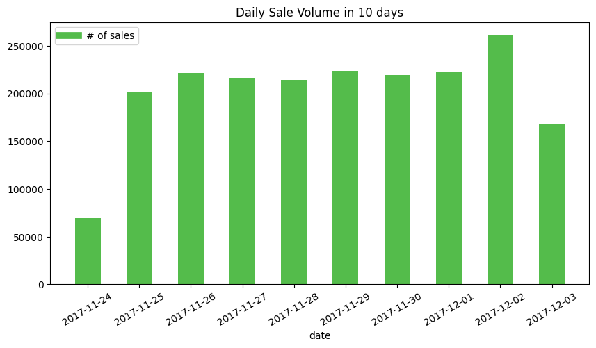
As PART II mentioned, due to the parsing issue, the UNIX time collected from GMT+8 time zone is interpreted to GMT-5 time zone, so part of sales conducted on 11-25 are binned to 11-24. One day shift to right, the sale volume based on a date shows a consistent invariance even encountering the weekends.
Hourly Sale Volume in 10 days
df_hourly_sales_volume = spark.sql("""
SELECT
    hour,
    SUM(CASE WHEN behavior = 'pv' then 0.1 else 0 end) as pv,
    SUM(CASE WHEN behavior = 'fav' then 0.1 else 0 end) as fav,
    SUM(CASE WHEN behavior = 'cart' then 0.1 else 0 end) as cart,
    SUM(CASE WHEN behavior = 'buy' then 0.1 else 0 end) as buy
FROM taobao
GROUP BY
    hour
ORDER BY
    hour
""").toPandas()
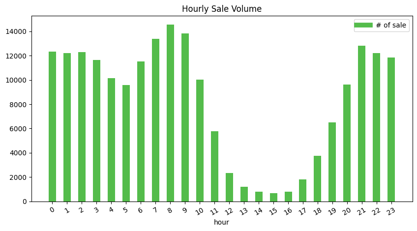
The UNIX time functions from Pyspark make the hour become the US time based on the local machine, so the hour shows in the figure should convert into the Beijing time as the sale are conducted in China region. e.g. 6 pm to 19:00
- Comparing with hourly behaviors distribution, the difference is in the period of time between 3 am (16:00) to 6 pm (19:00), the sale volume has a little decrease among all hours of the day.
- The peak has around 14000 sale volumes whereas the bottom has around 1000 sale volumes. The difference is around 14 times which is the same as the behavior distribution.
Sales Volume Ranking on item category
df_sales_volume_ranking_category = spark.sql("""
SELECT
    a.buy_times AS sales_volume,
    COUNT(a.category_id) AS category_num
FROM
    (SELECT
        category_id,
        COUNT(user_id) AS buy_times
    FROM
        taobao
    WHERE
        behavior='buy'
    GROUP BY
        category_id ) AS a
GROUP BY
    a.buy_times
ORDER BY
    category_num DESC;
""").toPandas()
sales_volume 	1 	2 	3 	4 	5 	6 	7 	8 	9 	10 	... 	1158 	3096 	18016 	1147 	458 	1326 	2015 	6354 	2782 	2203
category_num 	767 	448 	313 	268 	198 	195 	163 	133 	105 	97 	... 	1 	1 	1 	1 	1 	1 	1 	1 	1 	1
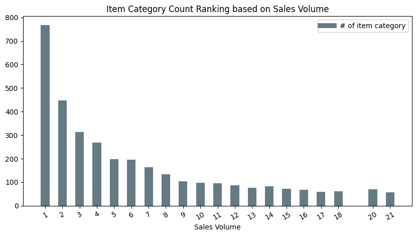
Based on the sale volume, we ranked the item categories’ count. The figure above shows there are almost 800 categories of items are sold only once among all users. The second place’s category of an item which sold twice counts around 450. The overall trend follows a logarithmic pattern in a descending prone.
Sales Volume Ranking on item id
df_sales_volume_ranking_item = spark.sql("""
SELECT
    a.buy_times AS sales_volume,
    COUNT(a.item_id) AS item_num
FROM
    (SELECT
        item_id,
        COUNT(user_id) AS buy_times
    FROM
        taobao
    WHERE
        behavior='buy'
    GROUP BY
        item_id ) AS a
GROUP BY
    a.buy_times
ORDER BY
    item_num DESC;
""").toPandas()
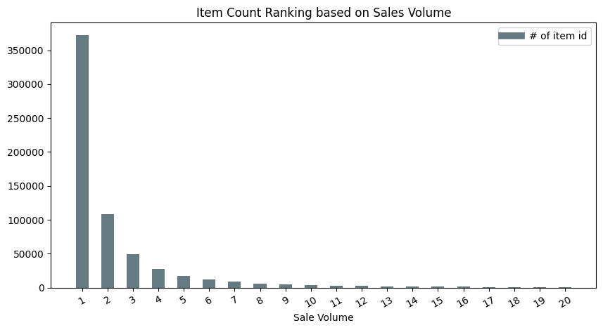
The second study on item id ranking based on the sale volume indicates a similar trend as to how it was performed with the item category rank. They both follow a logarithmic declining trend, but for the current item ranking trend, it is deeper. Over 350,000 items are sold once which takes a larger portion, whereas the items sold twice are only take 1/4 in the value.
Item id ranking vs Item category ranking (on Sale Volume)
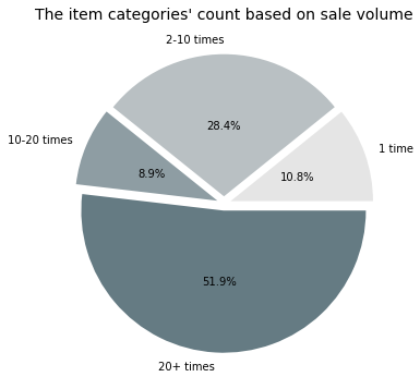
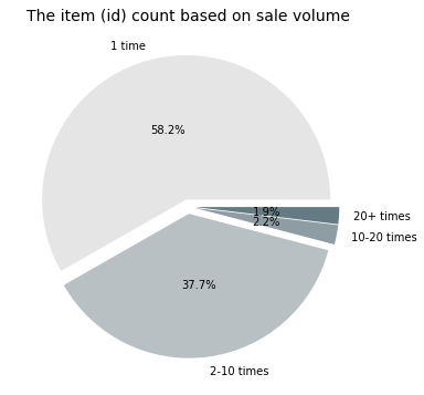
It is interesting to conduct the pie charts for both rankings and compare how much the portions take for different granularity of data tag. Much easy to understand, the category tag has fewer unique values than item id since one category can include multiple items, hence the portion for ranking would be different.
As seen from the figure on the left-hand side, half of the item categories have their belonging items sold 20+ times, as for those less popular item categories, one sold only once still takes 10 percent, these are the super unpopular item category. From the figure on the right-hand side, within the super unpopular item category, the items’ number overwhelmingly populates 58.2 percent among all items. Combined with the items which sold 2-10 times, it is interesting to see that most of the items (96 percent) of items are not popular at all, whereas only 2 percent of items are able to sell at least 20 times, in other words, getting into the transaction order.
For further mining processing, a possible direction is to cluster the item category based on the distribution of its item sale volume. One guess is there might have an item category that has 1 or 2 items specifically popular with almost no visit for the rest, or some item categories may exist that all items belonging to them are regular.
3. Recency, frequency, monetary value (RFM) Model
Recency, frequency, monetary value is a marketing analysis tool used to identify a company’s or an organization’s best customers by using certain measures. The RFM model is based on three quantitative factors:
- Recency: How recently a customer has made a purchase
- Frequency: How often a customer makes a purchase
- Monetary Value: How much money a customer spends on purchases
RFM analysis numerically ranks a customer in each of these three categories, generally on a scale of 1 to 5 (the higher the number, the better the result). The “best” customer would receive a top score in every category.
We take the above approach to category the users based on the rule with the last time buy behavior and frequency of buy behavior. Here are the rules:
R:score the user's recency based on the time difference from the buy behavior date to 17-12-03
difference > 7 score = 1
difference BETWEEN 5-7 score = 2
difference BETWEEN 3-4 score = 3
difference BETWEEN 0-2 score = 4

F:score the user's frequency based on the date of the buy behavior count
purchase once score = 1
purchase twice score = 2
purchase 3-10 times score = 3
purchase times > 10 score = 4
Since the table does not contain monetary info, hence ignore the monetary value.
Once having the scores of users’ Recency and Frequency, applying another rule to classify users into different group.
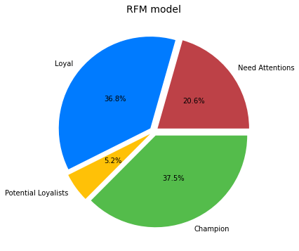
Champion:
FrequencyScore BETWEEN 3-4 AND RecencyScore BETWEEN 3-4

Loyal:
FrequencyScore BETWEEN 3-4 AND RecencyScore BETWEEN 1-2

Potential Loyalists:
FrequencyScore BETWEEN 1-2 AND RecencyScore BETWEEN 3-4

Need Attentions
FrequencyScore BETWEEN 1-2 AND RecencyScore BETWEEN 1-2
spark.sql("""
SELECT
    user_id,
    (CASE WHEN Rdiff >7 THEN 1
    WHEN Rdiff BETWEEN 5 AND 7 THEN 2
    WHEN Rdiff BETWEEN 3 AND 4 THEN 3
    WHEN Rdiff BETWEEN 0 AND 2 THEN 4
    ELSE NULL END ) AS RecencyScore
FROM
    (SELECT
        user_id,
        DATEDIFF('2017-12-03',max(date)) AS Rdiff
    FROM
        taobao
    WHERE
        behavior='buy'
    GROUP BY
        user_id)

""").createOrReplaceTempView("R1")

spark.sql("""
SELECT
    user_id,
    (case WHEN SaleVolume BETWEEN 1 AND 1 THEN 1
    WHEN SaleVolume BETWEEN 2 AND 2 THEN 2
    WHEN SaleVolume BETWEEN 3 AND 10 THEN 3
    WHEN SaleVolume >=11 THEN 4
    ELSE NULL END ) as FrequencyScore
FROM(
    SELECT
        user_id,
        COUNT(behavior) AS SaleVolume
    FROM
        taobao
    WHERE
        behavior='buy'
    GROUP BY
        user_id)
""").createOrReplaceTempView("F1")

df_RFM = spark.sql("""
SELECT
    user_id,
    RecencyScore,
    FrequencyScore,
    (CASE WHEN (FrequencyScore BETWEEN 1 AND 2)AND(RecencyScore BETWEEN 1 AND 2 )THEN 1
    WHEN (FrequencyScore BETWEEN 1 AND 2)AND(RecencyScore BETWEEN 3 AND 4 )THEN 2
    WHEN (FrequencyScore BETWEEN 3 AND 4)AND(RecencyScore BETWEEN 1 AND 2 )THEN 3
    WHEN (FrequencyScore BETWEEN 3 AND 4)AND(RecencyScore BETWEEN 3 AND 4 )THEN 4
    ELSE NULL END ) AS CustomerLevel
FROM
    (SELECT
        R1.user_id,
        R1.RecencyScore,
        F1.FrequencyScore
    FROM
        R1
    INNER JOIN
        F1
    ON
        R1.user_id=F1.user_id)
""").toPandas()

print(df_RFM)
        user_id  RecencyScore  FrequencyScore  CustomerLevel
0       1000240             4               3              4
1       1000280             4               2              2
2       1000665             4               3              4
3       1000795             4               2              2
4       1000839             4               3              4
...         ...           ...             ...            ...
672399   999498             2               1              1
672400   999507             4               3              4
672401   999510             4               3              4
672402   999616             2               1              1
672403   999656             3               1              2

[672404 rows x 4 columns]
Copyright @ 2021 Zizhun Guo. All Rights Reserved.
