YOLO Mechanism Part I: Input, Output, Encoding, Anchor Box, IoU, Decode, Confidence, NMS, Ground Truth，LOSS

Mechanism

Object Detection is a regression task that neural networks are required to output not only the predicting score and class for an object but also the bounding boxes. Figure 3 shows the basic mechanism of Yolo networks as the one-staged object detector.

Label y

As the figure[mechanism] shows, the output label is not the results output from the YOLO head layer, since the decode component would convert the bounding boxes’ encoding offsets into the real coordinates of the input image, Yolo Head works for filtering the real bound boxes and select ones that are expected to remain, therefore using the intermediate result – encodings as the labels ignores the additional operation and keeps the offsets as the normalized target values, which improved the efficiency to calculate the loss for the training process.

The shape of Input and Output

The input image is sized in (m, 416, 416, 3), whereas m represents the number of batches set by the practitioners, (416, 416) represents the pixel numbers for the weight and height of the input images, and the 3 represents the channels numbers as RGB channels.

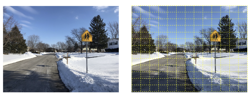
The output encoding is sized in (m, 26, 26, 21) or (m, 13, 13, 21), whereas m is the same as the input image, due to the object detector is FPN structured, therefore two scaled feature maps are extracted but the network, however, both (26, 26) and (13, 13) represents the same meaning, which is the cells numbers of the original images. Yolo algorithm requires the image to be divided into cells into variable scales so that to enable extracting objects in different distances since the objects at a far distance would be small-sized in the image which takes fewer numbers of pixels than the objects in closer distance.

Encodings

The encodings are fetched by the encoding process (see Encode in figure 3) while assigning the ground true samples during the training session or they are the intermediate results representing the extracted features process (see Feature Extractor in figure 3) which are output by the network backbone. The tensor size for the embeddings contains the same number of ranks of the input image but the actual features are thereby translated and embedded into the special object detection format.

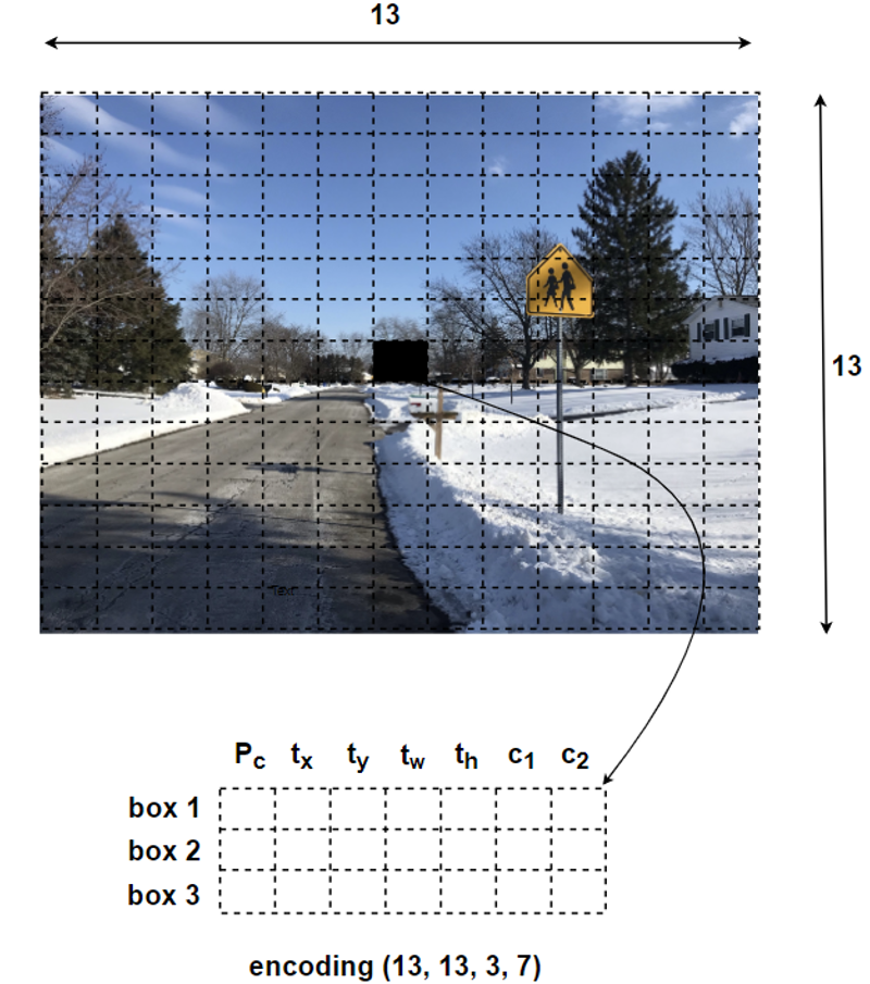
The last dimension number of the output encoding represents the list of bounding boxes along with the recognized classes. In our case, we have two classes: Traffic Signs and Stop Signs. As the specific flatten format of the encodings can be reorganized in a more meaningful way, from figure 5, the last element of the output encoding is 21, which also can be represented in (3, 7). The first element of 3 indicates that there are three anchor boxes, which are set to vary the scales of detecting results, whereas the number of 7 represents p_c, t_x, t_y, t_w, t_h, c_1, c_2.

• p_c : the confidence if it exists an object in current cell.
• t_x : the x coordinate of the offset to anchor box grid cell.
• t_y : the y coordinate of the offset to anchor box grid cell..
• t_w : the relative weight ratio for the anchor box.
• t_h : the relative height ratio for the anchor box.
• c_1 : the probability for the object being as a Traffic Sign.
• c_2 : the probability for the object being as a Stop Sign.

Anchor Box

The concept of anchor box was originally introduced by Faster RCNN. The anchor box (also known as the bounding box prior in the paper, and the anchor box is used later) is the statistics (using k-means) from all the ground truth boxes in the training set and the most frequently appearing box shapes and sizes in the training set. These statistical prior (or human) experiences can be added to the model in advance so that when the model is learning, the model converges quickly.

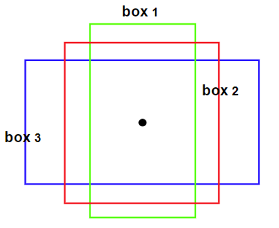
Another understanding about using anchor boxes is that the traditional object detection head used as the regressor can only detect one object. The performance for multiple object detection would be affected and interference due to the variant shape of the bounding boxes. To solve this issue, multiple regressors can be used which are all limited to specific detecting regions. To achieve such a mechanism, for each grid cell, there could set multiple anchor boxes in different shapes specifically in charge for detecting objects around the positions.

From 4.2 FPN and 5.3 Encodings parts, we have two routes of feature map output for each input image sample. Therefore, we have two features that are in tensors’ shape in (13, 13, 3, 7) and (26, 26, 3, 7). The third number 3 implies there are three anchor boxes that are used for specifying the regressors.

For the route feature maps in the shape of (26, 26, 3, 7), we select (23,27), (37,58), (81,82) sized bounding boxes as the anchor boxes. For the route feature maps in the shape of (13, 13, 3, 7), we select (81,82), (135,169), (344,319) as the anchor boxes.

As can be seen by the size values, for images divided into (26, 26) cells, each cell is smaller than the ones processed into (13, 13), hence the anchor boxes for (26, 26) cells are smaller in the number of pixels, whereas the (13, 13) cells have greater sized anchor boxes.

Intersection over Union for bounding boxes

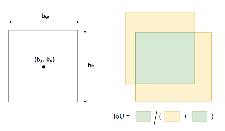
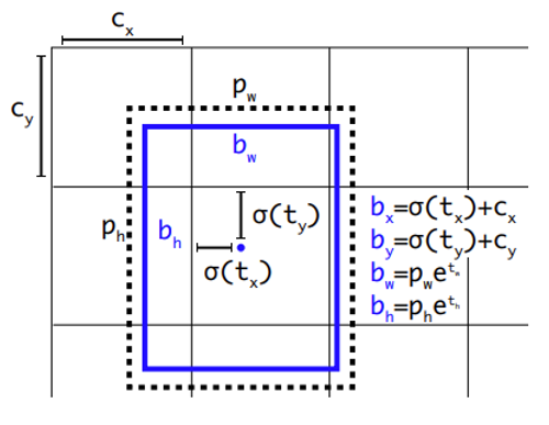
The bounding box is represented in a format of 4 numbers. In the different processes of the YOLO neural networks, the tensors of the bounding boxes are variant processed. For example, the bounding box values as the intermediate results that are produced after the encoding process are represented in the format of (t_x, t_y, t_w, t_h). This tensor cannot be directly used to reference the exact bounding box’s coordinates so that to use it as the prediction results. Therefore, such intermediate should be decoded into the real coordinates that have the midpoints, weights, and heights in size of the same scales of the real image. The actual bounding box is set to be in the format of (b_x, b_y, b_w, b_h) whereas b_x represents the bounding box mid point x-coordinate, b_y represents the bounding box mid point y-coordinate, b_w represents the weight of the bounding box and b_h represents the height of the bounding box.

Intersection over Union (IoU) is an evaluation metric that can be used in the prediction task of bounding boxes in values of ranges. The metric applies to all shapes of objects. In YOLO neural networks, it serves the same purpose by calculating the ratio between the intersection area over the union area to measure the accuracy of bounding boxes regressor.

Decode

As the anchor boxes have different sizes of the boxes, YOLO only predicts the bounding boxes in the format of (t_x, t_y, t_w, t_h) that bonds to different anchor boxes where each value represent the offsets and relative values, due to the model instability when in early training iteration[]. However, this form of coordinates does not affect the final location prediction. The decoding process would translate the temporary coordinates into the bounding boxes coordinates relevant to the real image size.

b_x= σ(t_x )+ c_x

b_y= σ(t_y )+ c_y

b_w=p_w e^(t_w )

b_h=p_h e^(t_h )

b_x and b_y represent the bounding box center coordinates, b_w and b_h represent the bounding box weight and height. t_x and t_y represent the level of the center point shifts reletively to the c_x and c_y which represent that the cell is offset from the top left corner of the image. The b_w and b_h represent the weight and height of the bounding box prior (also known as the anchor box).

The Decode process transforms the feature maps in the shape of (t_x, t_y, t_w, t_h) into the shape of (b_x, b_y, b_w, b_h), which makes it possible to not only take the advantage of anchor box mechanism but also by constraining the values of bounding boxes so that to make the network more stable.

Confidence Scores

YOLO defines the Confidence Scores as the product of the confidence and the Intersection of Union (IOU) of prediction and ground truth bounding boxes’ paris.

The Pr(〖Class〗_i

Object) from the equation in our case is c_1 and c_2. Therefore, the final confidence score is determined how much the overlapping ratio between the prediction and ground true bounding boxes and the object-specific probability.

Non-Max Suppression

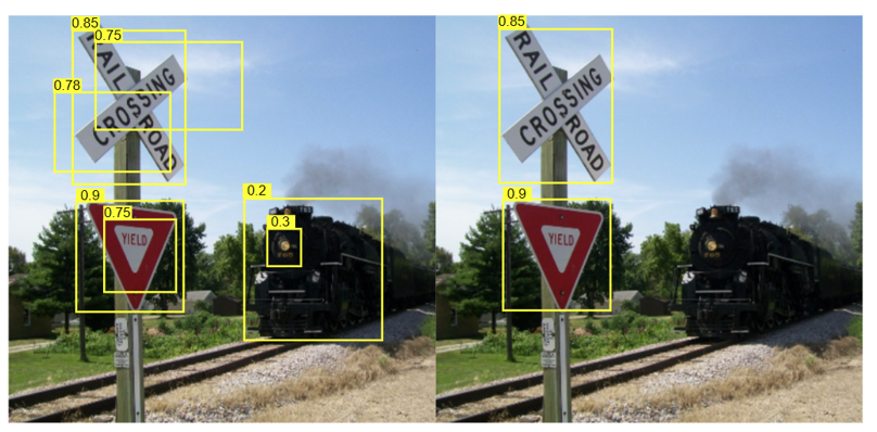
Non-maximum suppression (NMS) is an algorithm for removing non-maximum values. The simple understanding is to select all the partial substitutions by defining the part. In the process of object detection, a large number of candidate bounding boxes will be generated at the same object position. These candidate boxes may overlap with each other. In this situation, the NMS would first generates a detection box with the object detection confidence score, the detection boxes with the highest scores are replaced, and other detection boxes that have obvious overlap with the replaced detection boxes are suppressed.

The progress of the Non-maximum suppression algorithm : (1) Sort bounding box list by confidence scores; (2) Select the bounding box with the highest confidence score and add it to the final output list, and delete it from the bounding box list; (3) Calculate the area of all bounding boxes; (4) Calculate the IoU of the bounding box with the highest confidence score and other additional boxes; (5) Delete bounding boxes with IoU greater than the threshold; (6) Repeat the above process until the bounding box list is empty.

The image on the left is the result of the candidate boxes of YOLO detection. Each bounding box has a confidence score. If NMS is not used, multiple candidate boxes will appear such as duplicate bounding boxes on the same object and bounding boxes on other objects which should not be seen as the target objects. The image on the right-hand side is the result of using non-maximum suppression, which fits the expectation to have two bounding boxes attached on two traffic signs.

Ground Truth Boxes Assignment

Before the training session, one necessary step is to define the positive and negative cases for target variables for each image sample. It is essential to assign the ground true bounding box in the appropriate anchor box. Since each object, has only one corresponding bounding box for labeling but exists multiple anchor box regressors. The strategy is to calculate the IoU between ground true bounding box with each anchor box and select the anchor box with the greatest IoU as the target.

Loss

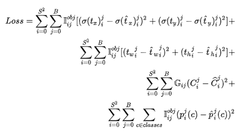
The loss function of YOLO v4 is mainly divided into three parts: bounding box regression loss, confidence loss and classification loss.

The S and B represent the grid cells number and the bounding box priors (anchor boxes) number. The value of I_ij^obj parameter decides whether count the loss of the bounding boxes. If I_ij^obj equals 1, it means that the predicting bounding box matches the current anchor box, whereas if it is 0, the loss does not take into account.

The G_ij plays a similar role as the I_ij^obj, it defines whether the confidence scores of the prediction result should be considered. For C_i^j =1, the predicted bounding box has the greatest IoU with ground truth box, hence C_i^j =0 for the cells of other anchor box types. One particular case is, the current anchor box which does not assign to detect a specific object class produces the IoU that is greater than the IoU threshold (YOLO paper is 0.5), G_ij would be 0 to neglect the loss calculation for it.

In the original YOLO paper[], the loss function employs sum-squared error for it is easy to calculate. In our project, we use the binary cross-entropy as the cost for each grid cell and bounding box prior.

---

Copyright @ 2021 Zizhun Guo. All Rights Reserved.