大数据分析课程:ROC曲线和1维分类 Data Mining: ROC curve and 1D classficication
Author: Zizhun Guo
作者:
写于:
- 1. Data set quantization
- 2. Main parts description
- ```
- 3. Comparison with Otsu’s method
- 4. Plotting: Costs based on Thresholds
- *Best threshold has been marked by red verticle line.
- 5. Plotting: ROC Curve
- 6. Conclusion
1. Data set quantization
    # location: HW02_Guo_Zizhun_Mentor.py/main

    # using floor binning method to quatize dat set
    data_ages = np.floor(df_snowfolks_data_raw['Age'] /bin_size_ages) \
                    * bin_size_ages  \
                    * df_snowfolks_data_raw['Class']

    data_heights= np.floor(df_snowfolks_data_raw['Height'] /bin_size_heights) \
                        * bin_size_heights \
                        * df_snowfolks_data_raw['Class']
2. Main parts description
2.1 Cost functions (minimal mixed cost)
    # location: HW02_Guo_Zizhun_Mentor.py/binary_classifier_1d

        FN = np.size(Class_A[Class_A > 0])                  # calculate the False Negatives
        FP = np.size(Class_B[Class_B < 0])                  # calculate the False Positives
        mixed_cost = FN + FP                                # calculate the mixed cost by adding up

        # Minimize the mistakes
        if mixed_cost < lowest_cost:
            lowest_cost = mixed_cost                              # update the minimal cost
            best_thresholds = [start]                           # update the best threshold
2.2 Selecting attribute
All attributes would be tested for selecting the final attribute as the standard attribute, which would be used in the trained program as the threshold.
    # location: HW02_Guo_Zizhun_Mentor.py/write_file

    # select attribute by comparing the lowest cost to decide the classify rule
    attribute = 'Age' \
        if lowest_cost_ages < lowest_cost_heights \
        else 'Height'
    threshold = best_thresholds_ages \
        if lowest_cost_ages < lowest_cost_heights \
        else best_thresholds_heights
3. Comparison with Otsu’s method
| CSV file | Program | Attibute | Threshold Value |
|---|---|---|---|
| Abominable_Data_For_1D_Classification__v93_HW3_720_final.csv | clustering: Otsu’s Method | Age | 46.0 |
| Ht | 145.0 | ||
| classification: Minimal number of misclassification | Age | 50.0 | |
| Height | 140.0 |
Table 1: Threshold result from running same data set on both homework program
It make no sense to compare the results produced by both programs since they serve different purposes (one is clustering, the other is classification). The clustering is a technique to organize the data into classes where the data which shares similarity would be grouped together. The classification is worked on label data where the class for each data is defined in the first place but to trained a program to do more classification work.
However, when scope down to cost function, Otus’s Method uses $cost = object(mixedVariance) + regularization$ as essential condition, whereas 1d Classifier, $cost = numberFalse Alarm + numberFalse Positive$.
Statistically, the Otus’ purpose is to assess the minimal distance between each points as its standard to group points, so the cost is calculated based on the spreading situation. The purpose of Classification for using total number of False Alarm and False positive is to make the splitting point as much accurate as possible by minimize the misclassification.
Besides, the attribute in values from two data set represent the same domain meaning, but in usage of data science, they are different by utilization. The classification would have labels attached on them, while clustering does not.
4. Plotting: Costs based on Thresholds
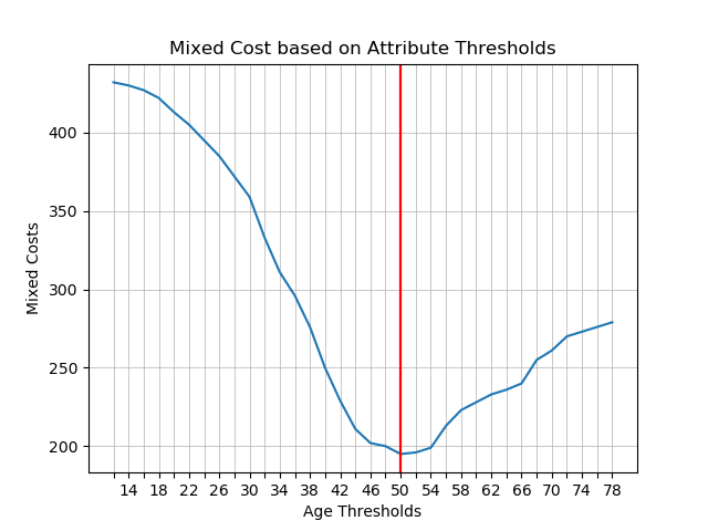
*Best threshold has been marked by red verticle line.
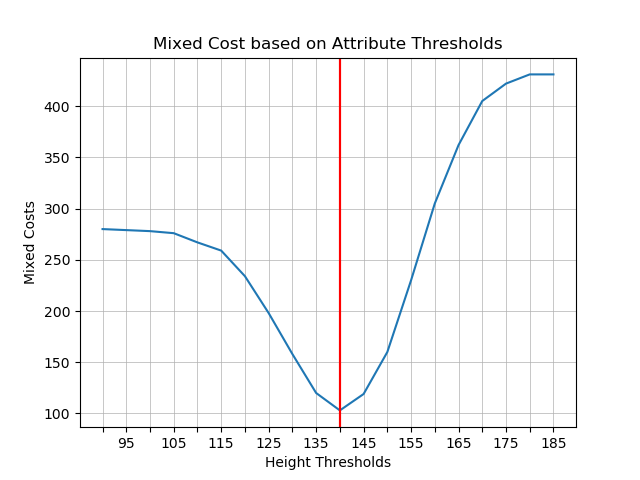
*Best threshold has been marked by red verticle line.
5. Plotting: ROC Curve
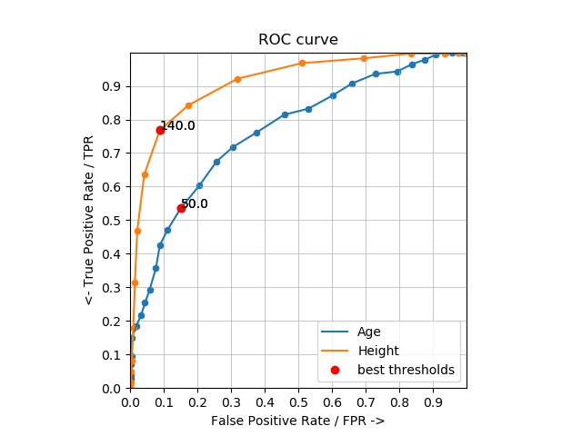
*Axes square by plt.gca().set_aspect('equal', adjustable='box')
*Indication showed by red dots with best threshold annotated
*There might be multiple best thresholds for a single attribute, conclusion would be posted in Part 6.
6. Conclusion
6.1 What did I discovered?
The domain knowledge should be collected before setup the Cost Function. It determines which specific side to classify data set whereas if attribute is Height, Bhutan is on the left.
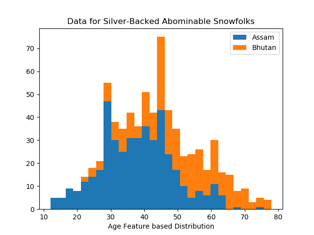
*if Attribute is Age, Bhutan is on the right of historgram.
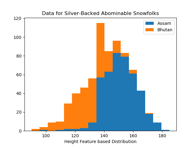
*if Attribute is Height, Bhutan is on the left of historgram.
The Splitting Point (Best thresholds) tends to be centerlized at points range where most samples lying on (condense part).
6.2 Which attribute did I use?
Height It has the best ROC curves, all points of the height line is above ones on age line, which indicating less number of misclassification since they were calculated by sum of FAR and FNR, best point is expected to have high y-coordinate and low x-coordinate.
For scenerios that has disparate distribution on both Age distribution and Height distribution. The program is smart enough to detect which attribute to select.
See Implementation at 2.3 Selecting attribute
6.3 Were the results what I expected?
|Labels|Prediction|Results| |—|—|—| |+|+|Correct| |-|-|Correct| |-|-|Correct| |-|-|Correct| |+|-|Wrong| |-|-|Correct| |-|-|Correct| |-|-|Correct| |+|+|Correct| |+|+|Correct| |+|-|Wrong| |+|-|Wrong| |-|-|Correct| |-|+|Wrong| |+|+|Correct| |+|+|Correct|
Table 2: Classification Accuracy
Summary: correct: 12; wrong: 4; total: 16
$CorrectnessRate = numCorrect / TotalNum = 12/16 = 0.75$
The accuracy of current classifer model is 75%. Validated by validation CSV file. This is my expectation, since the homework documents said there would be no perfect classification in this case. So 75% is a number which somehow can indicate that.
6.4 What was surprising?
What maybe shocked is the accuracy is low. It will give a wrong prediction every 3 out of 4 given data record. However, since this is a simple classification model, it does not surprise much. On the other hand, if the accuracy for one model is too high more than expectation, this could be wrong, since higher accuracy towards one specific data set tends make it overfitting. - by the concept of Accuracy Paradox.
6.5 Was there anything particularly challenging?
Selection of data structure to contain data that required for each plotting task.
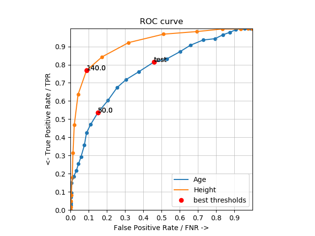
As homework document described, “Caution, there may be more than one of them”, so there must implemente a data strutrue that is able to contains all roc points with lowest cost, and can be plotted them in the same ROC curve figure. So here is how to implemented in homework:
    # Data structure [[(x1, y1), threshold1],...,[(xn, yn), thresholdn]]
    for roc_point_with_lowest_cost in roc_points_with_lowest_cost:
        for roc_point_with_lowest_cost_duplicate in roc_point_with_lowest_cost:
            plt.plot(roc_point_with_lowest_cost_duplicate[0],
                    roc_point_with_lowest_cost_duplicate[1],
                    'ro')
            plt.annotate(roc_point_with_lowest_cost_duplicate[2],
                        (roc_point_with_lowest_cost_duplicate[0],
                        roc_point_with_lowest_cost_duplicate[1]))
So data structure contains these info looks like this: $ [[(x1, y1), threshold1],…,[(xn, yn), thresholdn]]$ A list of list that contains a coordinate tuple and a matching best threshold
Break Ties This is the other name for descibing this siatution. So in order to break ties, a regularization could be added to help select the best threshold. Here in my cases, my regularization is set to be a check condition whereas if the attribute selected is Age, it selects the lowest best threshold, while if it is Height attribute, so to choose the highest best threshold.
This is designed towards classifying as much Bhutan animals as possible so while the best thresholds have the same number of misclassification, the one with highest True Positive Rate would be selected even though the higher False Positives Rates followed. The purpose is taking the greatest probablity to classify correct Bhutan, so the misclassfied Assam is what we have to take in the same time.
In codes implementation, the first best threshold would be select if distribution is Age-like, while the last best threshold would be chosen if distribution is built under attribute of Height.
    # location: HW02_GUO_Zizhun_trained.py/main

    # based on domain knowledge to choose which side to classify as Assam or Bhutan
    if attribute == 'Age':
        for val in data:
            if val <= threshold[0]: # select first best threshold
                print('- 1')
            else:
                print('+ 1')
    if attribute == 'Height':
        for val in data:
            if val <= threshold[np.size(threshold) - 1]: # select the last best threshold
                print('+ 1')
            else:
                print('- 1')
6.6 Did anything go wrong?
ROC curve without domain knowledge may casue single side classification.

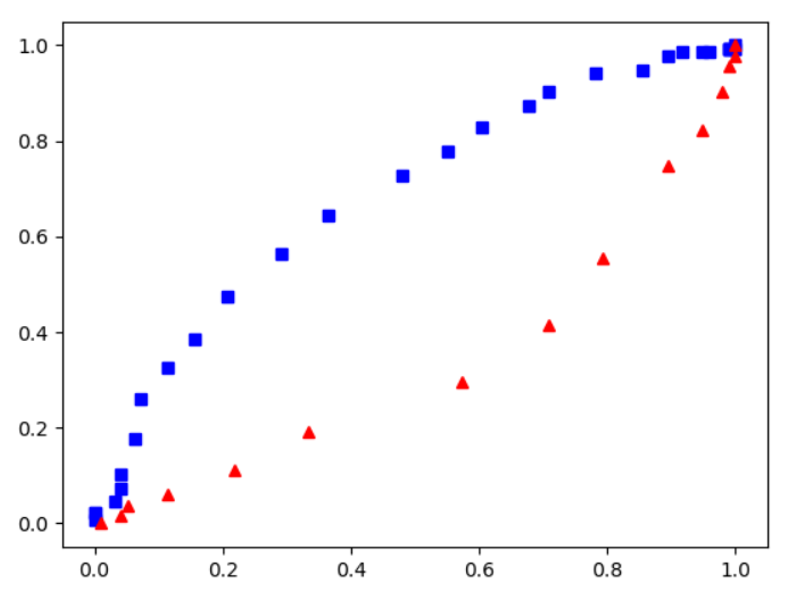
At the begining of development, I did not know about the distribution of the dataset, so I assumed all Brutan animals spreaded as larger ages and greater heights, but only after I plot the rough ROC curve (to observe the shape) did I realize I had missed the information of distribution. Later then after plotting the histogram, it helped to imporved the classification function.
This works is used for Course CSCI720. Do not spread it if it is unauthorized.